Minimal Clinically Important Difference (MCID) of Effect Sizes other than Mean Difference

Introduction

The evaluation of effect size or measures of association traditionally relied on P value testing against null hypotheses, assuming no difference or association. However, evaluating effect size based solely on statistical significance has been criticized by the scientific community.1,2 In response to this critique, it has become standard methodology to assess the clinical significance of an effect size along with the P value in medical research. In practice, a researcher is recommended to report both a P value less than 0.05 and an effect size exceeding the minimal clinically important difference (MCID) to assert a meaningful difference or association between two clinical measurements. Examples of MCID of mean difference (MD) include a 4-point change in the St. George Respiratory Questionnaire total score for patients with chronic obstructive pulmonary disease and a 4.1-point change in the Unified Parkinson’s Disease Rating Scale total score.3,4

In addition to the MD, various effect sizes are used in clinical studies, such as hazard ratio (HR), risk ratio (RR), odds ratio (OR), absolute risk difference (ARD), correlation coefficient (r), and area under the receiver operating characteristic curve (AUC), to quantify difference and association between two clinical measurements and to assess diagnostic ability.5–8 Evaluating these effect sizes based solely on the P value is not optimal. However, the MCID has not been established for these effect sizes. Therefore, a researcher often questions whether an improvement in AUC from 0.80 to 0.85 is clinically meaningful or not. Many researchers have been hoping for the establishment of the study-level MCID of a variety of effect sizes that patient-level assessment cannot be applied for.

Establishing an MCID for these effect sizes may be challenging for some reasons. First, the MCID of the effect sizes, such as HR and AUC, cannot be directly equated to a “slight improvement” or “small but noticeable deterioration” in a patient. Furthermore, some of these effect sizes are on a non-interval scale,9,10 meaning that the same numerical change in the effect size has different implications depending on the baseline value. For instance, the difference in Pearson’s product r between 0.0 and 0.2 is not equivalent to that between 0.8 and 1.0.

In this manuscript, we propose methods to establish study-level MCID, by converting Cohen’s d into major effect sizes, namely HR, RR, OR, ARD, r, and AUC. We also advocate study-level MCIDs for each of these effect sizes.

Methods and Examples

Distribution Method

Two popular methods are employed to determine the MCID of MD for a certain measurement: the anchor method and the distribution method.11–15 The anchor method establishes MCID based on the smallest difference in the measurement that patients can perceive, typically equating to descriptions such as “slightly improved” or “slightly deteriorated,” using a ladder in seven classes. The distribution method estimates MCID using specific standardized mean difference (SMD) values, known as Cohen’s d, calculated as “the mean difference (MD) between two groups divided by the pooled standard deviation (SD),” corresponding to 0.5 (large MCID), 0.3 (medium MCID), or 0.2 (small MCID).11–15 Cohen’s d has a range when used as the MCID, and several factors must be considered when selecting an appropriate value. For example, for outcomes with significant clinical implications, such as survival prognosis, the small Cohen’s d of 0.2 is often chosen. Although the distribution method has been criticized for its reliance on statistical conventions and experimental methodologies, it is widely accepted in the field of clinical research.

We do not delve into which d value is the most preferred as an MCID, but our method is applicable to any d value, such as 0.1 or 0.8. In the following sections, we often use d = 0.5, amongst 0.5, 0.3, and 0.2, as an example because of the ease of illustrating figures but not because d = 0.5 is the preferred choice.

When two groups have sufficiently large sample sizes and equal SDs, the pooled SD used in Cohen’s d calculation is equal to the SD of each group. Based on this assumption, the SD of each group and the pooled SD are considered interchangeable hereafter.

Hazard Ratio

HR is an effect size used in survival time analysis to compare the follow-up duration to an event such as death or heart attack. It is derived from the Cox proportional hazards model: a value greater than 1 indicates increased risk, less than 1 suggests decreased risk, and equal to 1 implies no difference between the groups.8 Here, we define the MCID of the HR that corresponds to a survival time difference associated with a specific Cohen’s d value. Both Mantel–Haenszel and Log-rank methods are applicable to our proposal; the HR value hereafter is calculated from the log-rank method.

The Cox proportional hazards model incorporates the concept of censoring; however, for simplicity, we assume no censoring. “Survival data” are usually a combination of a continuous variable for the follow-up duration and a binary variable for event/censoring data. Thus, ignoring censoring simplifies survival data to a single continuous variable representing survival time. When two groups have survival time distributions that follow a normal distribution with the equal SD and the between-group SMD of 0.5, i.e., d = 0.5 (Fig. 1A), the corresponding survival curves shown in Fig. 1B result in HRs of 1.56 or 0.64. This conversion was not based on a calculation using a specific formula but rather on a statistical software implementation of the Cox proportional hazards model (R, “survival” library, “coxph” function, Breslow method for tie data). In clinical research, survival time typically does not follow a normal distribution but is instead right-skewed. Therefore, we present another example wherein the natural log transformation (ln) of survival time is normally distributed (Figs. 1C–1E). The survival curves seem to be a typical presentation with weak early event delay due to the inclusion of patients in good condition accompanied by an HR of either 1.56 or 0.64 (Fig. 1E). Note that the survival time is processed as if it were an ordinal variable in the survival time analysis, and any transformation that preserves the patient order does not alter the HR (Figs. 1B and 1E).

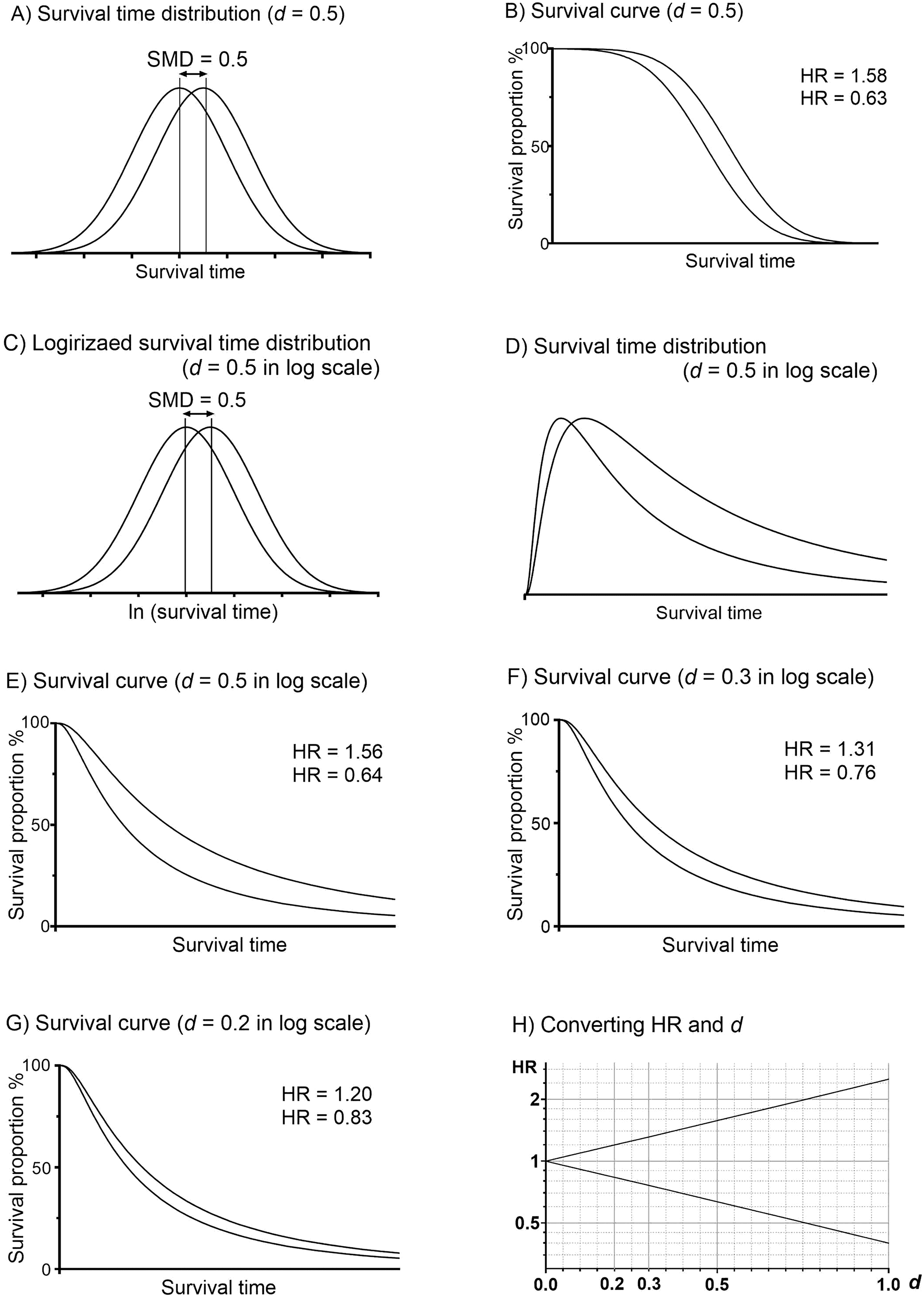
Figure 1. MCID of the hazard ratio. MCID, minimal clinically important difference; HR, hazard ratio; d, Cohen’s d; ln, natural logarithm transformation; SMD, standardized mean difference.

For a d value of 0.3, the corresponding HRs are 1.31 and 0.76 (Fig. 1F), and for a d value of 0.2, the HRs are 1.20 and 0.83 (Fig. 1G). Fig. 1H may be useful for converting between HR and Cohen’s d.

Example with real data

A trial was planned to compare adjuvant pembrolizumab versus placebo in resected stage III melanoma. The sample size was determined based on a detectable difference, an HR of 0.7 for recurrence-free survival.16 The detectable difference, closely related to the concept of MCID, is the smallest effect size that a study is designed to detect. Most trials typically set the detectable difference for an HR between 0.6 and 0.85 based on empirical evidence, which almost corresponds to Cohen’s d between 0.2 and 0.5 (Figs. 1E–1G).

In a non-inferiority randomized trial, the “FOLFIRI” regimen was compared to the “OFF” regimen for treating patients with metastatic pancreatic adenocarcinoma.17 The sample size was calculated based on the non-inferiority margin, an HR of 1.5, which approximately corresponds to a Cohen’s d value of 0.5 (Fig. 1E). A non-inferiority margin is the predefined maximum allowable difference considered clinically negligible, and its concept is similar to that of the MCID. Non-inferiority margins in the range of 1.2 to 1.6 are usually selected for trials, which are comparable with our proposal (Figs. 1E–1G).

A systematic review and meta-analysis of data from 12,251 patients demonstrated that sodium-glucose cotransporter two inhibitor administration reduced the risk of first hospitalization for heart failure, with an HR of 0.72.18 This represents a substantial reduction, exceeding the “medium” MCID (HR of 0.76, Cohen’s d of 0.3, Fig. 1F). Therefore, we agree that the drug is effective in preventing hospitalization due to heart failure. The article also mentioned that the treatment “significantly” reduced all-cause mortality, with an HR of 0.92 (95% confidence interval 0.86–0.99). However, an HR of 0.92 did not meet the “small” MCID criteria (HR of 0.83, d = 0.2, Fig. 1G). It is important to note that the large sample size in the meta-analysis makes a clinically insignificant difference become statistically significant.

Effect Size for Binary Variables

Some researchers propose a default RR of 0.8 or 1.25 as representing small effect sizes.19 However, we should modify MCID for RR based on risk in the control group, which is often called the “baseline risk.” If we accept that the fixed MCID of the RR is 1.25, when the event rate, or risk, in the control group is 90%, the event rate in the experimental group should be at least 112% to exceed the MCID, which is impossible. Therefore, the MCID for the RR should be flexible, adjusting closer to 1 as the risk in the control group increases. Similarly, the MCID of ARD should be flexible. We propose flexible MCID for the effect sizes of RR, OR, and ARD. The experimental group may be termed the study group, exposure cohort, or intervention arm according to the study background.

The probit model defines the probability of an “event” in a binary event/non-event variable by the cumulative distribution function of a normal distribution. For instance, assuming that the hemoglobin level is normally distributed, we can define an event “anemia” as hemoglobin <13.0 g/dL and non-event “without anemia” as hemoglobin ≥13.0 g/dL. Assuming the risk in the control group was 16%, the cutoff Z-score for the control group (Zctrl) is calculated as Zctrl = ${\Phi }^{-1}$ (risk in control group) = ${\Phi }^{-1}$ (0.16) = −1, where $\Phi$ represents the cumulative distribution function, and ${\Phi }^{-1}$ represents inverse cumulative distribution function, also known as probit function (Fig. 2A). MCID for RR, OR, and ARD will be calculated from the risk in control and experimental groups where the risk in the experimental group = $\Phi$ (${\Phi }^{-1}$ (risk in control group) ± d) = $\Phi$ (Zctrl ± d). This is equivalent to d = |${\Phi }^{-1}$ (risk in experimental group) − ${\Phi }^{-1}$ (risk in control group) |. Cohen’s d represents the SMD between the two normal distributions determining two risks (Figs. 2B and 2C). For example, given that d = 0.5 and the risk in the control group is 16%, the risk in the experimental group is calculated as follows: $\Phi$ (${\Phi }^{-1}$ (0.16) ± 0.5) = $\Phi$ (−1 ± 0.5) = $\Phi$ (−0.5) = 0.31 or $\Phi$ (−1.5) = 0.07 (Figs. 2B and 2C). Based on the control group risk of 16% and experimental group risk of 31%, d = |${\Phi }^{-1}$ (0.31) − ${\Phi }^{-1}$ (0.07) | = | (−0.5) − (− 1) | = 0.5 (Fig. 2C).

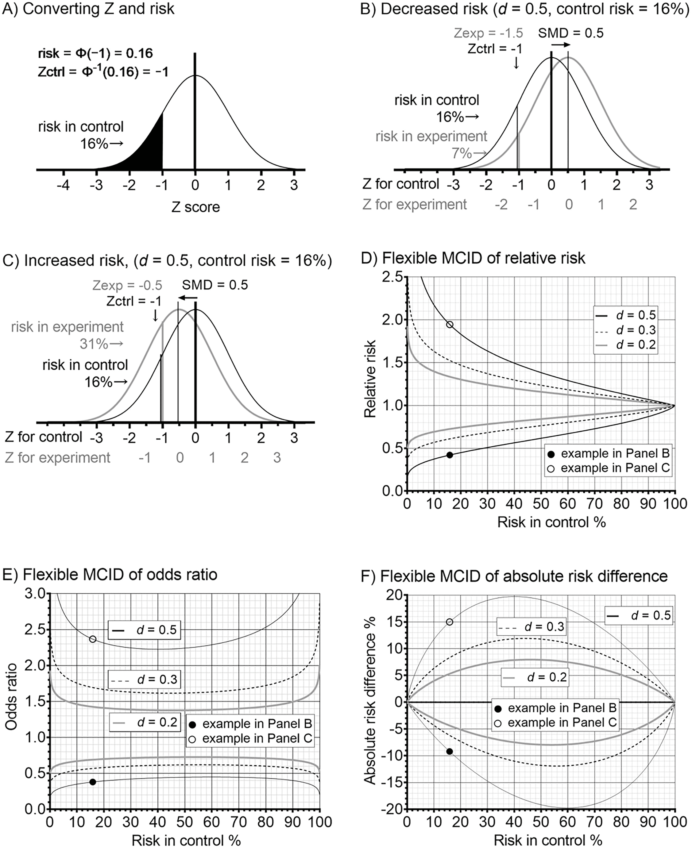
Figure 2. Flexible MCID of binary effect sizes. MCID, minimal clinically important difference; d, Cohen’s d; SMD, standardized mean difference; Zctrl, Z for control; Zexp, Z for experiment; $\mathrm{\Phi }$, cumulative distribution function. Panels D, E, and F: A closed and open circles explain the examples in panels B and C, respectively.

Relative risk

RR, also known as the risk ratio, compares the probability of an event occurring in an experimental group with that in a control group.7 An RR greater than 1.0 suggests a higher risk in the experimental group, while an RR less than 1.0 indicates a reduced risk.

In the example shown in Fig. 2B, the risk in the control group is 16%, and the risk in the experimental group is 7%, yielding the MCID of RR = 0.42 (Fig. 2D). In the example shown in Fig. 2C, the MCID of the RR is calculated as $\Phi$ (−0.5)/$\Phi$ (−1) = 31%/16% = 1.94 (Fig. 2D). Fig. 2D shows the MCID of RR across a range of risks in the control group from 0 to 1, with d values of 0.5, 0.3, and 0.2. For example, based on d = 0.2, when the risk in control is 30%, MCID is either 0.78 or 1.24.

Odds ratio

Odds represent the ratio of the probability of an event occurring to the probability of it not occurring.7 The OR compares the odds between the two groups, where an OR value greater than 1 indicates higher odds in the experimental group. The OR and RR share a similar concept, and their values are close to each other when baseline risk is low.

We use the probit model to determine the flexible MCID of OR, as we did for RR. For example, with a risk of 16% in the control group and d = 0.5, the risk on the increased side in the experimental group is 31% (Fig. 2C). Thus, the MCID of OR is 2.37 (Fig. 2E).

Some use the formula ln (OR) = d·$\pi /\sqrt{3}$ to convert an OR into d,20 which yields fixed ORs of 2.48, 1.72, and 1.44, corresponding to d values of 0.5, 0.3, and 0.2, respectively. These values closely match our proposed MCID of OR when the control risk is between 10% and 90%. However, to apply a consistent method with RR and ARD, we chose to adopt the probit model instead.

Absolute risk difference

ARD is an “absolute” effect size, unlike the relative effect sizes such as RR or OR.7 It represents the actual difference in event risk between the two groups, providing valuable information for clinical decision-making regarding intervention.

Based on the same example, where the risk in the control group is 16%, d = 0.5, and the risk in the experimental group is 31% (Fig. 2C), the MCID of ARD is calculated to be 15% (Fig. 2F).

Example with real data

A total of 502 patients with recurrent or metastatic cervical cancer were randomly assigned to receive tisotumab vedotin monotherapy or traditional chemotherapy.21 The confirmed response rates, as one of the secondary endpoints, were 17.8% in the tisotumab vedotin monotherapy arm and 5.2% in the chemotherapy arm (OR 4.0). According to Fig. 2E, an OR of 4.0 exceeds even the large MCID (d = 0.5, baseline risk = 5.2%, OR 2.7). To put it another way, d = ${\Phi }^{-1}$ (0.178) − ${\Phi }^{-1}$ (0.052) = (−0.92) − (−1.63) = 0.71 is larger than 0.5. It can, therefore, be concluded that tisotumab vedotin clinically meaningfully improved the confirmed response rate compared to traditional chemotherapy.

A phase III trial was designed to assess neoadjuvant short-course radiotherapy followed by camrelizumab and chemotherapy in locally advanced rectal cancer.22 To estimate sample size, the researchers assumed pathological complete response rates of 18% in the control arm and 36% in the experimental arm. According to the proposed formula, d = |${\Phi }^{-1}$ (0.36) − ${\Phi }^{-1}$ (0.18)| = |(−0.36) − (−0.92)| = 0.56. Therefore, the detectable difference is almost compatible with the large MCID defined by d = 0.5.

A recent systematic review, based on 15 published studies, claimed that male sex was associated with higher risk of admission due to respiratory syncytial virus-related acute lower respiratory infection (OR 1.23, 95% confidence interval 1.19–1.27).23 Supported by the large sample size, P < 10−30 suggested high statistical significance. However, regardless of the baseline risk and choice of d, an OR of 1.23 does not meet the MCID (Fig. 2E). Statistical significance and clinical significance may diverge in meta-analyses.

Correlation Coefficient

The correlation coefficient, denoted as r, quantifies the upward or downward trend between two variables.6 Pearson’s product-moment coefficient measures the linear correlation, while Spearman’s rank coefficient assesses the monotonic relationships between ranks. The r value ranges from −1 to 1, wherein 1, −1, and 0 mean perfect upward correlation, perfect downward correlation, and no correlation, respectively.

Cohen’s d is not directly applicable to r, primarily because r is not on an interval scale. Another issue is that r is the effect size for the association but not for the difference. However, d can be applicable to r after converting it into an SMD through the following formula: SMD = f (r) = 2·r/√(1 − r2), r = f−1(SMD) = √(SMD2/(SMD2 + 4)).24 This conversion formula can be understood in the following way. When two groups of normally distributed continuous variables with a specific SMD are assigned dummy group labels of 0 and 1, the coefficient r quantifies the association between group labels and the continuous value. Fig. 3A shows that SMD = 0.87 corresponds to an r-value of 0.4 based on the conversion above. Note that the continuous value shown in the Y axis of Fig. 3A is a hypothetical number used to convert r to SMD, and they are entirely unrelated to the two variables usually used to calculate r. Besides, an SMD of 0.87 does not correspond to Cohen’s d value of 0.87. Fisher’s Z transformation is used to map the correlation coefficient r, which ranges from −1 to 1, to the entire range of real numbers. However, Fisher’s Z transformation is not intended for directly converting a single r value into SMD.

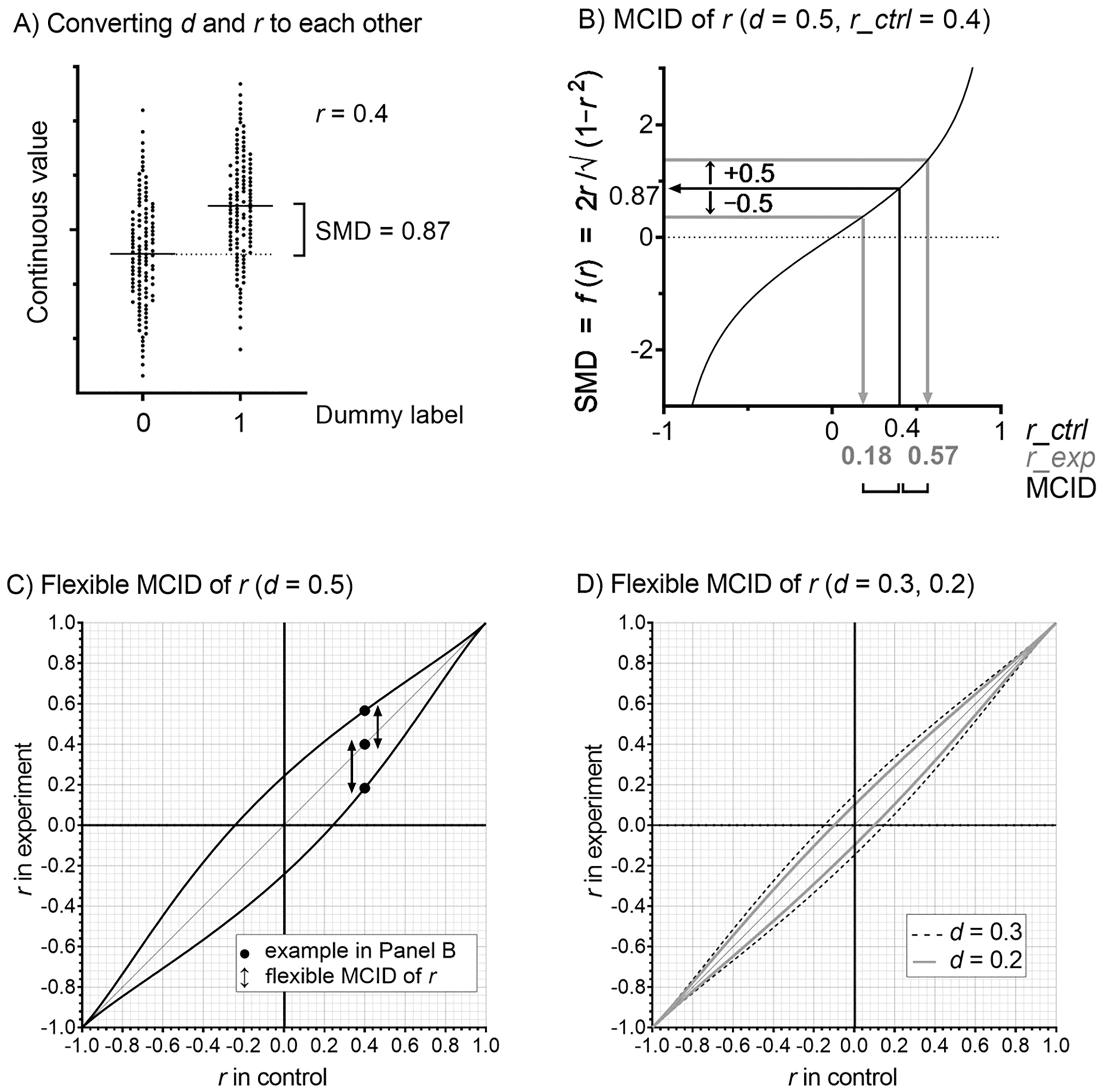
Figure 3. Flexible MCID of r. f (r) = 2·r/√(1 − r2). MCID, minimal clinically important difference; r, correlation coefficient; r_ctrl, r for control test; r_exp, r for experimental test; d, Cohen’s d; SMD, standardized mean difference.

Because r is not on an interval scale, a fixed MCID cannot be applied for r across the range of −1 to 1. Therefore, we introduce a novel concept, “flexible MCID of r,” for a varying r value that ranges from −1 to 1. We define the flexible MCID of r by the difference corresponding to d in the f-transformed scale (Fig. 3B). In other words, the MCID of r is the difference between r for control ($r\mathrm{\_}ctrl$) and r for experimental ($r\mathrm{\_}exp$): $r\mathrm{\_}exp$ = f −1(f ($r\mathrm{\_}ctrl$) ± d). This is to say, d = |f ($r\mathrm{\_}exp$) − f ($r\mathrm{\_}ctrl$)|. For example, d = 0.5 and $r\mathrm{\_}ctrl$ = 0.4, which leads to $r\mathrm{\_}exp$ = 0.18 and 0.57, as shown in Figs. 3B and 3C. The MCIDs are 0.22 and 0.17 for the lower and upper sides, respectively. Fig. 3C depicts the proposed flexible MCID of r employing the d = 0.5 criteria and control r. Fig. 3D shows those for d = 0.3 and 0.2.

Assuming $r\mathrm{\_}ctrl$ = 0, d values of 0.5, 0.3, and 0.2 are translated to r values of 0.24, 0.15, and 0.10, respectively. These coefficients are closely aligned with the generally recognized thresholds for negligible correlations, |r| < 0.1 or < 0.2.25,26

Example with real data

For patients with cardiac arrest, it is necessary to interrupt chest compressions to measure systolic blood pressure. However, since stopping chest compressions decreases the chances of successful resuscitation, a method for estimating systolic blood pressure without interrupting chest compressions is needed. In a study of 35 cardiac arrest patients, it was demonstrated that peak systolic velocity measured by ultrasound (r = 0.71) had a significantly better correlation with systolic blood pressure than the traditional end-tidal CO2 (r = 0.31; Fisher Z-transformation, P < 0.001).27 Our interest lies in how the difference between $r\mathrm{\_}ctrl$ = 0.31 and $r\mathrm{\_}exp$ = 0.71 is interpreted clinically. Cohen’s d, given by f (0.71) − f (0.31) = 2.02 − 0.65 = 1.37, far exceeds the large MCID (d = 0.5), suggesting that the difference has substantial clinical significance.

Area Under the Receiver Operating Characteristic Curve

The AUC serves as an indicator of diagnostic test accuracy and how effectively an index test predicts a binary reference standard, typically the presence or absence of a disease. A higher AUC indicates better performance, with values of 1 and 0.5 representing perfect classification and random test.5 ΔAUC is calculated by comparing the AUC of the control index test and the experimental index tests against the reference standard test (gold standard, the answer),

Under the assumption that reference (+) and (−) groups have normally distributed continuous variables in the index test with the same SD and the specific between-group SMD (Fig. 4A), the index test distinguishes the two groups with AUC = $\Phi$ (SMD/√2), wherein $\Phi$ is the normal cumulative distribution function.28,29 Note that this between-group SMD does not suggest Cohen’s d. For an assumed SMD of 1.5, AUC = $\Phi$ (1.5/√2) = 0.86 (Fig. 4B and 4C).

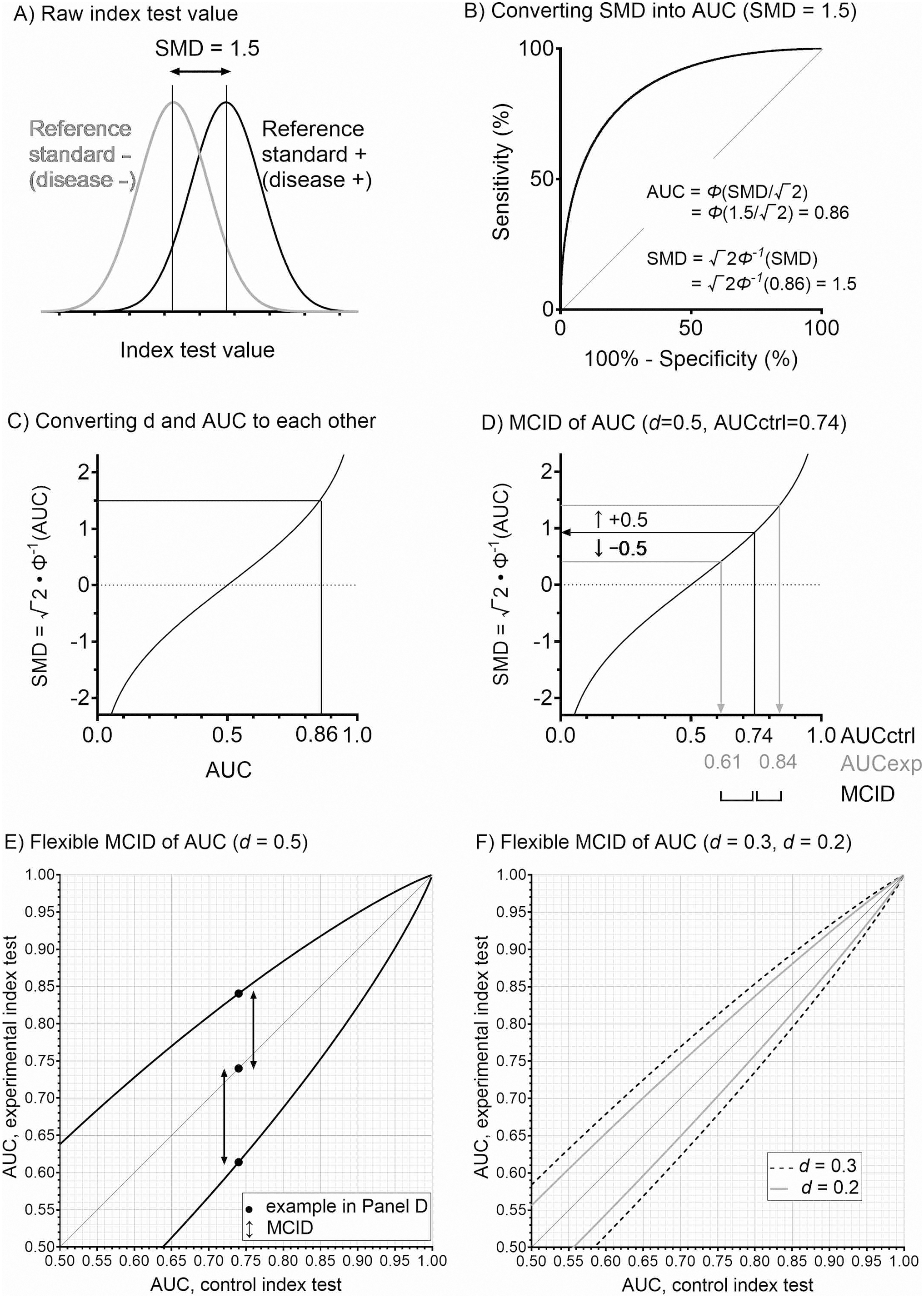
Figure 4. Flexible MCID of AUC. MCID, minimal clinically important difference; AUC, the area under the receiver operating characteristic curve; d, Cohen’s d; SMD, standardized mean difference.

A fixed ΔAUC as MCID across varying AUC is not appropriate because it is not on an interval scale. For instance, ΔAUC of 0.1 has a different impact when comparing AUC of 0.5 and 0.6 and when comparing 0.8 and 0.9. We introduce the “flexible MCID of AUC,” as we did for the correlation coefficient r. We define the flexible MCID by the difference between AUC for the control test (AUCctrl) and experimental test (AUCexp) when the latter is given below: AUCexp = $\Phi$ ((√2 · ${\Phi }^{-1}$ (AUCctrl) ± d)/√2). This is equivalent to d = |√2 · ${\Phi }^{-1}$ (AUCexp) − √2 · ${\Phi }^{-1}$ (AUCctrl) |. For example, when d = 0.5 and AUCctrl = 0.74; then, √2 · ${\Phi }^{-1}$ (AUCctrl) = 0.91 (Fig. 4D). Then, AUCexp are 0.61 and 0.84, denoting MCID of 0.13 and 0.10 for the lower and upper sides, respectively, as shown in Figs. 4D and 4E. Fig. 4E depicts the AUCexp and proposed flexible MCID for control AUCctrl ranging from 0.5 to 1 based on the d = 0.5 criteria. Fig. 4F shows those for d = 0.3 and 0.2.

Example with real data

Because postcardiotomy veno-arterial extracorporeal membrane oxygenation requires substantial medical resources, it is necessary to predict in-hospital mortality to select appropriate patients. An individual patient data meta-analysis with 1,269 cases was conducted.30 Compared to a model with six explanatory variables predicting in-hospital mortality (AUC = 0.679), another model that additionally included lactate as an explanatory variable had a better ability to predict in-hospital mortality with the statistical significance (AUC = 0.731; DeLong test P < 0.0001). Here, d = √2 ·${\Phi }^{-1}$ (AUCexp) − √2 ·${\Phi }^{-1}$ (AUCctrl) = √2 ·${\Phi }^{-1}$ (0.731) − √2 · ${\Phi }^{-1}$ (0.679) = 0.22 is slightly larger than the small MCID (Fig. 4F, d = 0.2). Whether the observed difference in AUC is clinically meaningful depends on the choice of d among 0.2, 0.3, and 0.5.

Discussion

For MD, the MCID can be determined using either an anchor- or distribution-based method. The anchor-based approach focuses on individual perceptions of change, making it well-suited for patient-level MCID. Conversely, the distribution-based method, which utilizes statistical measures such as SMD, is designed for study-level MCID. These methods are mutually complementary. Because effect sizes other than the MD, such as HR, RR, OR, ARD, r, and AUC, cannot be conceptualized at the patient level, the distribution method was selected for our proposal. Our primary innovation lies in converting SMD expressed by Cohen’s d into other effect sizes, introducing a flexible MCID for non-linear effect sizes, and linearizing non-linear metrics using transformation functions.

Cohen proposed benchmarks of 0.2, 0.5, and 0.8 SD to represent small, medium, and large differences, respectively.31 Usually, the distribution method denotes the MCID as the difference corresponding to d from 0.2 to 0.5.32 Our current proposal focuses on a method for converting Cohen’s d into the MCID of effect sizes other than the MD, setting aside the choice among d = 0.5, 0.3, and 0.2. We should not mindlessly select a single MCID value, but the MCID should be decided based on the research context, patient variability, metrics in the control assessment, and outcome types.11–15 For example, an HR of 0.83 derived from d = 0.2 may be a reasonable criterion for a hard and vital outcome such as all-cause death in RCT. However, A HR of 0.64 derived from d = 0.5 may be suitable for softer outcomes, surrogate endpoints, and possibly biased observational studies.

Commenting on the limitations of this study: First, we cannot establish a clear standard for determining whether 0.2, 0.3, or 0.5 is the most appropriate Cohen’s d for the MCID. Additionally, some assumptions underlying the calculation of the MCID, such as the normality of the distributions and the equality of variances between the two groups, may not always be valid. Despite these limitations, the MCID values we propose are consistent with clinical judgment and experimental MCID selection, as demonstrated using several real data examples, and provide a useful general guideline.

Additionally, it provides useful MCIDs for various effect sizes, which is particularly valuable for avoiding comparisons between two groups based solely on the P-value, a practice that has been increasingly discouraged in recent years.1,2 The proposed MCID is useful not only for interpreting treatment effects in single RCTs and observational clinical studies but also in an epidemiological survey and in systematic reviews and meta-analyses, where the large number of patients makes statistical significance easily attainable. The proposed MCID is also useful for determining the effect size in the sample size estimation and deciding the non-inferiority margin for a non-inferiority trial. We hope that our approach to determining the MCID will serve as the guidance for designing and interpreting future clinical research that deals with HR, RR, OR, ARD, r, and AUC.

Acknowledgment

None.

Funding

None.

Authors’ Contributions

NH contributed to the conception of the work and drafting of the manuscript. SY contributed to the conception of the work and critical revision of the manuscript. YU, TK, TM, and TY were involved in the critical revision of the manuscript. All authors provided final approval of the manuscript and take full accountability for its content.

Data Availability

Not applicable.

Institutional Review Board Statement

Not applicable.

Conflict of Interest Disclosures

The authors report no conflicts of interest in this work.

Supplemental Information

Supplemental information for this article can be found online at https://sup.jclinque.com/api/articles/53/download-suppl.

References

[1] Amrhein V, Greenland S, McShane B. Scientists rise up against statistical significance. Nature. March 2019;567(7748):305–307. doi:10.1038/d41586-019-00857-9.

[2] Wasserstein RL, Lazar NA. The ASA’s statement on p-values: context, process, and purpose. Am Stat. May 2016;70(2):129–131. doi:10.1080/00031305.2016.1154108.

[3] Jones PW. St. george’s respiratory questionnaire: MCID. COPD. March 2005;2(1):75–79. doi:10.1081/COPD-200050513.

[4] Shulman LM, Gruber-Baldini AL, Anderson KE, et al. The clinically important difference on the unified Parkinson’s disease rating scale. Arch Neurol. January 2010;67(1):64–70. doi:10.1001/archneurol.2009.295.

[5] Akobeng AK. Understanding diagnostic tests 3: receiver operating characteristic curves. Acta Paediatr. May 2007;96(5):644–647. doi:10.1111/j.1651-2227.2006.00178.x.

[6] de Winter JC, Gosling SD, Potter J. Comparing the pearson and spearman correlation coefficients across distributions and sample sizes: a tutorial using simulations and empirical data. Psychol Methods. Septemper 2016;21(3):273–290. doi:10.1037/met0000079.

[7] Schechtman E. Odds ratio, relative risk, absolute risk reduction, and the number needed to treat–which of these should we use? Value in Health. September–October 2002;5(5):431–436. doi:10.1046/J.1524-4733.2002.55150.x.

[8] Spruance SL, Reid JE, Grace M, Samore M. Hazard ratio in clinical trials. Antimicrob Agents Chemother. August 2004;48(8):2787–2792. doi:10.1128/aac.48.8.2787-2792.2004.

[9] Asuero AG, Sayago A, González AG. The correlation coefficient: an overview. Crit Rev Anal Chem. 2006;36(1):41–59. doi:10.1080/10408340500526766.

[10] Berkson J. Application of the logistic function to bio-assay. J Am Stat Assoc. 1944;39(227):357–365. doi:10.2307/2280041.

[11] Copay AG, Subach BR, Glassman SD, et al. Understanding the minimum clinically important difference: a review of concepts and methods. Spine J. September–October 2007;7(5):541–546. doi:10.1016/j.spinee.2007.01.008.

[12] Jaeschke R, Singer J, Guyatt GH. Measurement of health status. Ascertaining the minimal clinically important difference. Control Clin Trials. December 1989;10(4):407–415. doi:10.1016/0197-2456(89)90005-6.

[13] Mouelhi Y, Jouve E, Castelli C, et al. How is the minimal clinically important difference established in health-related quality of life instruments? Review of anchors and methods. Health Qual Life Outcomes. May 12, 2020;18(1):136. doi:10.1186/s12955-020-01344-w.

[14] Norman GR, Sloan JA, Wyrwich KW. Interpretation of changes in health-related quality of life: the remarkable universality of half a standard deviation. Med Care. May 2003;41(5):582–592. doi:10.1097/01.MLR.0000062554.74615.4C.

[15] Pettersson S, Lundberg IE, Liang MH, et al. Determination of the minimal clinically important difference for seven measures of fatigue in Swedish patients with systemic lupus erythematosus. Scand J Rheumatol. May 2015;44(3):206–210. doi:10.3109/03009742.2014.988173.

[16] Eggermont AMM, Blank CU, Mandala M, et al. Adjuvant pembrolizumab versus placebo in resected stage III melanoma. N Engl J Med. May 2018;10(19):1789–1801. doi:10.1056/NEJMoa1802357.

[17] Modest DP, Heinemann V, Schütt P, et al. Sequential therapy of refractory metastatic pancreatic cancer with 5-FU/LV/irinotecan (FOLFIRI) vs. 5-FU/LV/oxaliplatin (OFF). The PANTHEON trial (AIO PAK 0116). J Cancer Res Clin Oncol. July 1, 2024;150:332. doi:10.1007/s00432-024-05827-x.

[18] Vaduganathan M, Docherty KF, Claggett BL, et al. SGLT-2 inhibitors in patients with heart failure: a comprehensive meta-analysis of five randomised controlled trials. Lancet. September 3, 2022;400(10354):757–767. doi:10.1016/S0140-6736(22)01429-5.

[19] Schünemann H, Brożek J, Guyatt G, et al. GRADE Handbook, 5.2.4.2 Imprecision in in systematic reviews; 2013. Accessed February 1, 2023. https://gdt.gradepro.org/app/handbook/handbook.html.

[20] Chinn S. A simple method for converting an odds ratio to effect size for use in meta-analysis. Stat Med. November 2000;30(22):3127–3131. doi:10.1002/(ISSN)1097-0258.

[21] Vergote I, González-Martín A, Fujiwara K, et al. Tisotumab vedotin as second- or third-line therapy for recurrent cervical cancer. N Engl J Med. July 4, 2024;391(1):44–55. doi:10.1056/NEJMoa2313811.

[22] Lin ZY, Zhang P, Chi P, et al. Neoadjuvant short-course radiotherapy followed by camrelizumab and chemotherapy in locally advanced rectal cancer (UNION): early outcomes of a multicenter randomized phase III trial. Ann Oncol. 2024;35(10):882–891. doi:10.1016/j.annonc.2024.06.015.

[23] Deng S, Cong B, Edgoose M, et al. Risk factors for respiratory syncytial virus-associated acute lower respiratory infection in children under 5 years: an updated systematic review and meta-analysis. Int J Infect Dis. September 2024;146(Suppl 1):107125. doi:10.1016/j.ijid.2024.107125.

[24] Mathur MB, VanderWeele TJ. A simple, interpretable conversion from pearson’s correlation to cohen’s for d continuous exposures. Epidemiol. March 2020;31(2):e16–e18. doi:10.1097/EDE.0000000000001105.

[25] Mukaka MM. Statistics corner: a guide to appropriate use of correlation coefficient in medical research. Malawi Med J. September 2012;24(3):69–71.

[26] Schober P, Boer C, Schwarte LA. Correlation coefficients: appropriate use and interpretation. Anesth Analg. May 2018;126(5):1763–1768. doi:10.1213/ANE.0000000000002864.

[27] Haddad G, Margius D, Cohen AL, et al. Doppler ultrasound peak systolic velocity versus end tidal carbon dioxide during pulse checks in cardiac arrest. Resuscitation. February 2023;183:109695. doi:10.1016/j.resuscitation.2023.109695.

[28] Kraemer HC, Frank E, Kupfer DJ. How to assess the clinical impact of treatments on patients, rather than the statistical impact of treatments on measures. Int J Methods Psychiatr Res. June 2011;20(2):63–72. doi:10.1002/mpr.340.

[29] Salgado JF. Transforming the area under the normal curve (AUC) into cohen’s d, Pearson’s rpb, odds-ratio, and natural log odds-ratio: two conversion tables. Eur J Psychol Appl Legal Context. 2018;10(1):35–47. doi:10.5093/ejpalc2018a5.

[30] Biancari F, Kaserer A, Perrotti A, et al. Hyperlactatemia and poor outcome After postcardiotomy veno-arterial extracorporeal membrane oxygenation: an individual patient data meta-Analysis. Perfusion. July 2024;39(5):956–965. doi:10.1177/02676591231170978.

[31] Cohen J. Statistical power analysis for the behavioral sciences, revised edition; Chapter 2, The t test for means; 2.2, The effect size index d, pp. 20–26. NY: Academic Press; 1977.

[32] Guyatt GH, Osoba D, Wu AW, et al. Methods to explain the clinical significance of health status measures. Mayo Clin Proc. April 2002;77(4):371–383. doi:10.4065/77.4.371.

APPENDIX

Excel file: MCID calculator.

Copyright: © 2024 Horita et al. This work is licensed under a Creative Commons Attribution 4.0 International License, which permits unrestricted use, distribution, and reproduction in any medium, provided the original work is properly cited.